When every story sounds the same
A story does not persuade alone. Its funding speed depends on what surrounds it, when it appears, and why the neighbouring stories sound alike. We tested that across 1,453,846 Kiva loans, 2016–2025.
The puzzleFunding got faster while the stories got more alike
Which is the opposite of what a simple "too much competition" story predicts.
Median funding time fell from 121.2 hours in 2024 to 68.1 in 2025, a 44 % drop — and over the same period the platform had fewer active same-sector loans but higher narrative homogeneity than at any point in the decade. Lower volume, more sameness, yet faster funding. Whatever similarity does to lender attention, it clearly does not do it on its own.
So we stopped asking "does crowding slow funding" and asked a sharper question: does similarity only bite when it creates live substitutes? That is an interaction, not a main effect, and it is testable.
The methodRebuild the market each lender actually faced
For every focal loan we reconstruct the choice set as it stood the moment that loan went live — same sector, same week, same country, so that the only thing differing is the narrative environment.
| Channel | Pool | Volume | Homogeneity | Saturation |
|---|---|---|---|---|
| Current | loans live on the platform at that same moment | C = log(1 + active same-sector count) |
H = mean cosine of the focal narrative to that pool | C×H |
| Recent | loans posted 35–65 days earlier, 7-day half-life weights | V | G | V×G |
Why 35 days. Training-period fundraising duration P95 = 826.891 h = 34.45 days, rounded up. Every loan in the lagged pool therefore has a ≥ 95 % chance of having finished fundraising before the focal loan appeared — it cannot mechanically drive the focal outcome.
Two details that matter more than they look. Similarity is not brute-forced pairwise but computed through
the exact identity mean cosine = focal vector · mean pool vector, checked against
brute-force recomputation to a maximum absolute error of 2.909e−14 against a 1e−9
threshold. And every variable definition was
frozen before any
result was inspected, so nothing downstream could be tuned to taste.
Before trusting itWe spent the first week trying to break our own design
This is the part we would want read first.
Before touching the real data we generated 20,000 synthetic loans with the true coefficients planted in
them, along with an unobservable sector-week demand shock, 72 lending partners, rising template share, and a
true signal deliberately placed in the use field rather than description. Then we ran
the proposed pipeline against it and scored every estimate against an answer key the pipeline was never
allowed to read.
It failed.
| Specification | Estimate of C (crowding) | Planted truth |
|---|---|---|
| Active pool — our own headline spec | 0.444 | 0.138 |
| Active pool, controlling for the true shock (cheating benchmark) | 0.089 | 0.138 |
| Mirror pool — built from posting time only, so outcomes cannot contaminate it | 0.107 | 0.138 |
The headline specification overstated crowding by roughly 3×, and the cheating benchmark proved the bias came from exactly the shock we had planted. The mirror pool recovered a nearly unbiased estimate without knowing the shock existed — at the cost of attenuating homogeneity (H falls from a true 0.170 to 0.054). That is an explicit trade, and we state it as one: accept coefficient attenuation to remove endogeneity bias.
Fourteen methodology components were scored this way. Three earned their place, four were permanent no-ops, five were written in a way that would mislead, and two actively made the estimates worse. One was a genuine logic hole: our placebo rule would have failed a perfectly correct design. Cutting the dead weight roughly halved the analysis workload without losing a single defensible conclusion.
You can reproduce all of it in about 90 seconds, with no competition data:
git clone https://github.com/Bella10142003/kiva-narrative-saturation.git
cd kiva-narrative-saturation
pip install numpy pandas scipy scikit-learn
bash run_demo.sh
The findingSimilarity hurts when it creates live substitutes
| Estimate | Reading | |
|---|---|---|
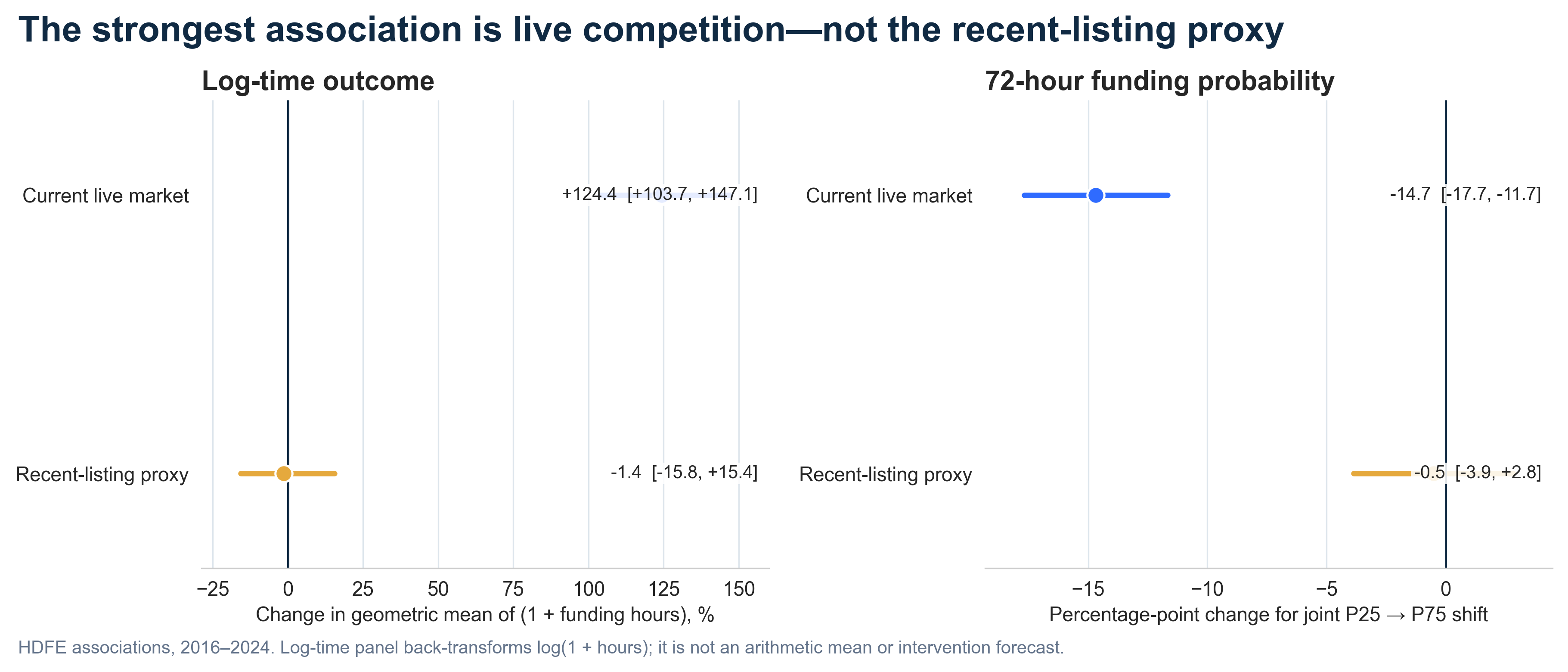
Current pool (C×H) | β = 0.1017, p = 0.0033 | Moving volume and homogeneity together from P25 to P75 lengthens funding time by +124.35 % [103.71, 147.08] and drops the 72-hour funding probability by 14.68 pp [−17.69, −11.67] |
Recent pool (V×G) | β = 0.0417, p = 0.0037 | Survives and strengthens to 0.0585 (p = 0.0007) once lending-partner template language is stripped — but the joint scenario is −1.42 % [−15.81, +15.43], crossing zero, because βV > 0 and βG < 0 cancel |
So the two channels behave differently, and we report them differently. The live-competition channel is a strong, robust association. The wear-out proxy has a real local interaction but we decline to promote it into an average effect, because the joint scenario it implies does not clear zero.
Stress testHow much of it survives
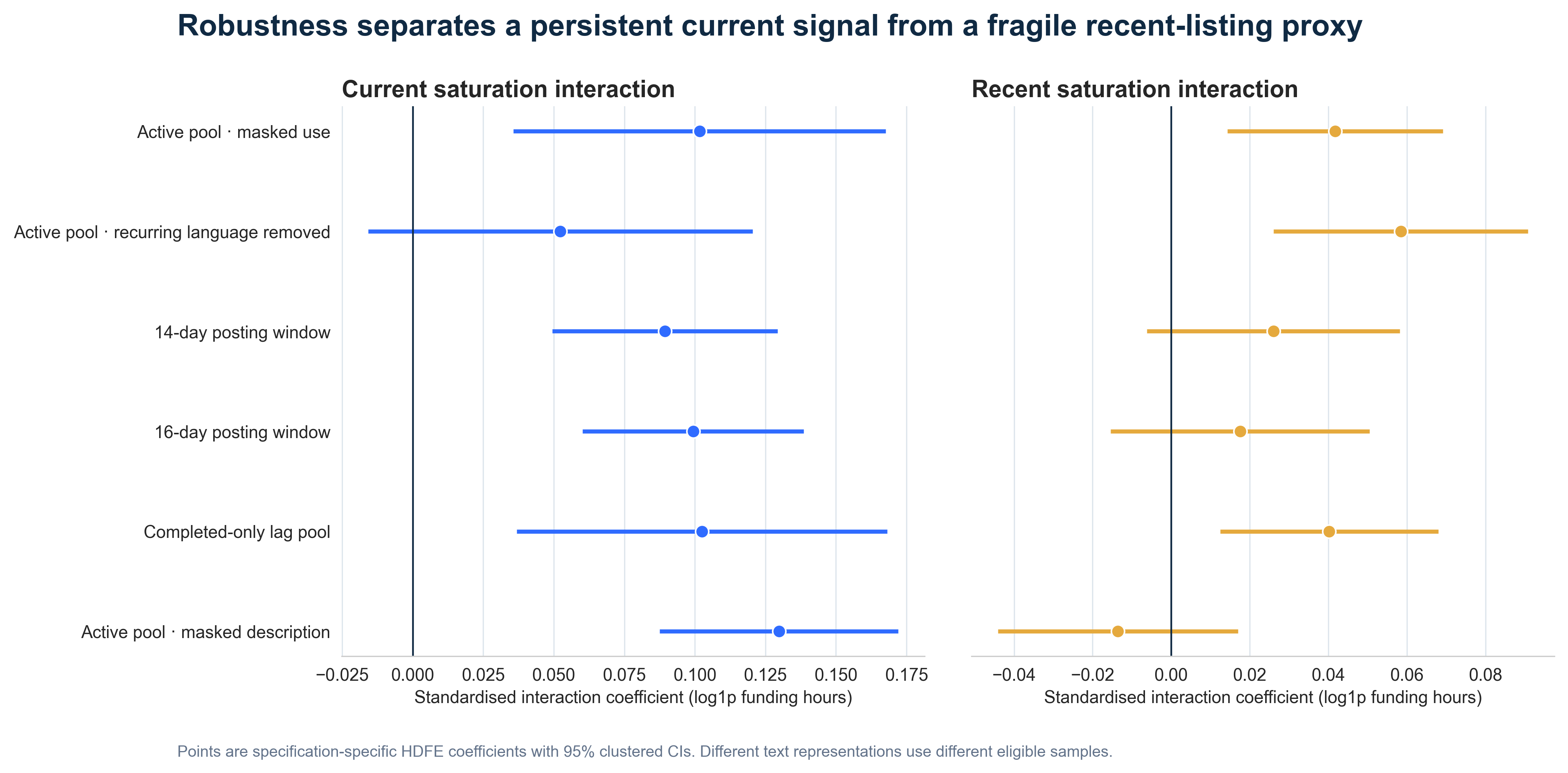
use, recurring language removed, 14- and
16-day posting windows, completed-only lag pool, masked description.The current-pool signal holds across all six. The recent-pool proxy is the fragile one, and the figure says so rather than hiding it.
Then the harder test: 2025 was held out for the entire project and never touched. On it, adding the narrative features made prediction worse — R² 0.5524 → 0.5370, AUC 0.8986 → 0.8921, six of seven metrics degraded, only log-loss marginally improved.
We report that as found. An explanatory association inside a fixed-effects structure is simply not the same thing as incremental predictive power on a future year, and the gap between the two is the whole reason the recommendation below is an experiment rather than a product.
The line we will not crossWhat this cannot be used for
The data has no impressions, no ranking, no clicks, no lender identity and no partner ID. Every record in
the extract already has a raisedDate, so true right-censoring cannot even be identified. These are
conditional associations in observational data, and we say so on every slide that carries a number.
- No borrower scoring. Do not deploy this as a ranking, approval, penalty or auto-rewriting tool.
- No moral reading. A saturation score is not borrower quality or creditworthiness.
- No subgroup targeting. Calibration gaps persist across gender and sector; those diagnostics are guardrails, not levers.
- No "tell it louder". The burden belongs to the platform's templates and scheduling, not to the borrower.
Two gaps are still open and recorded in the review log rather than papered over: RQ2's joint V/G/V×G test is not yet written into an artifact, and RQ4's within-sector versus platform-wide question has no output. Final QA stands at 19 of 20 gates.
The recommendationValidate first, then operate
Because the holdout did not support a scoring model, the recommendation is deliberately smaller than the finding: use current saturation as an experiment trigger, at the market level, and test two platform-side levers — staggered listing and diversified exposure, and partner-approved template alternatives. Randomisation units, guardrails, MDE and stopping rules are pre-registered before anything ships.
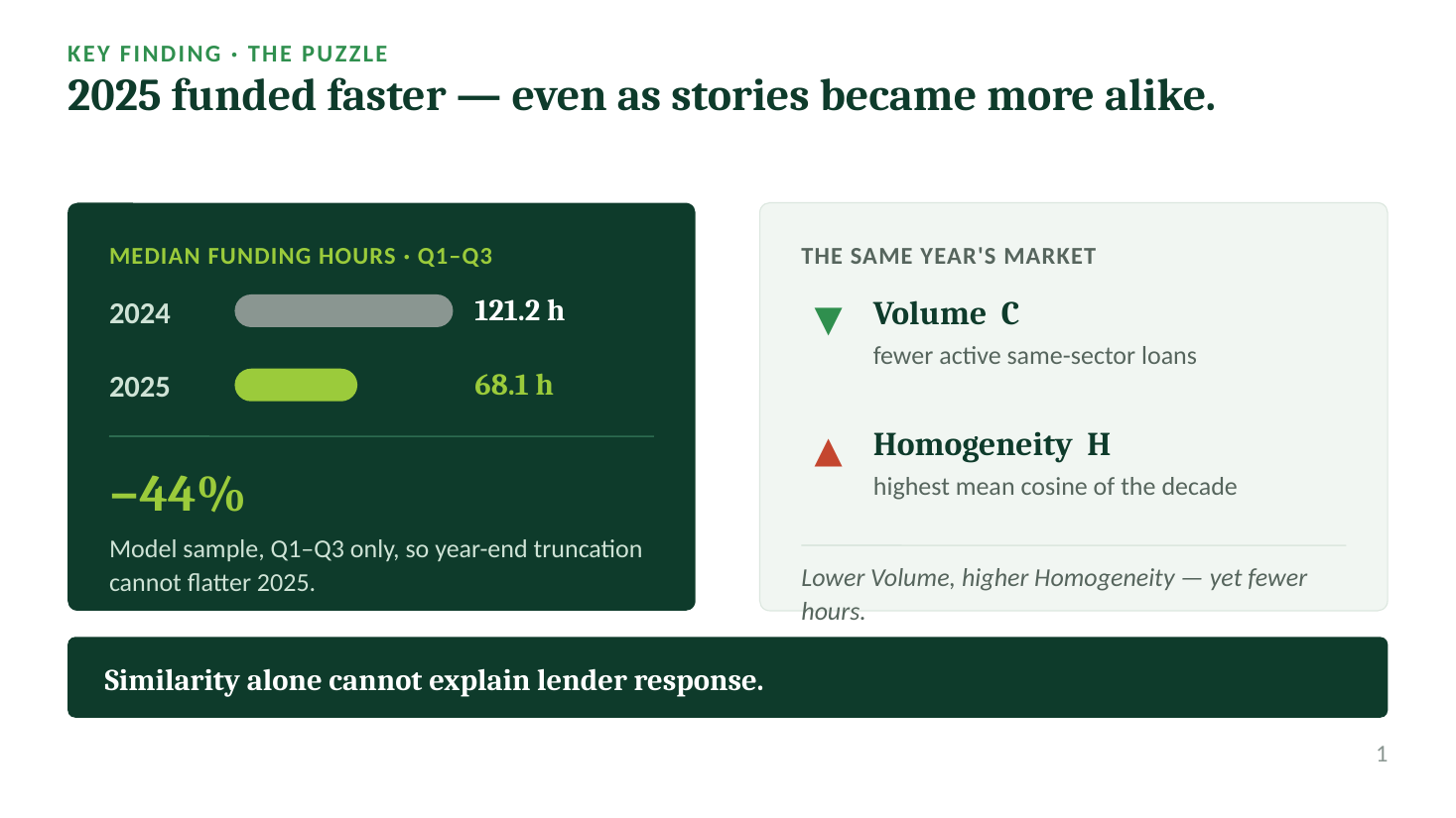 The puzzle — 2025 funded faster even as stories became more alike
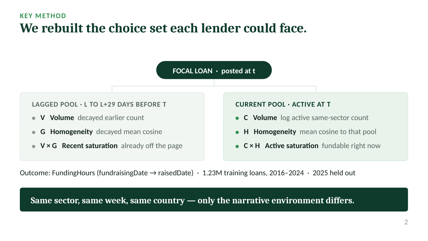 The method — rebuilding the choice set each lender could face
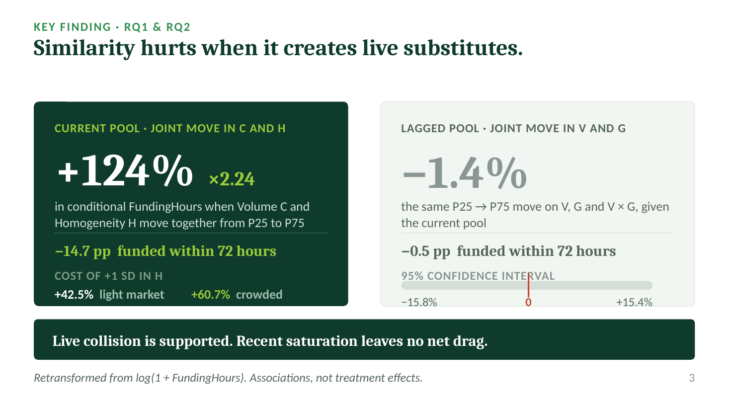 The finding — +124 % on the current channel, no net drag on the recent one
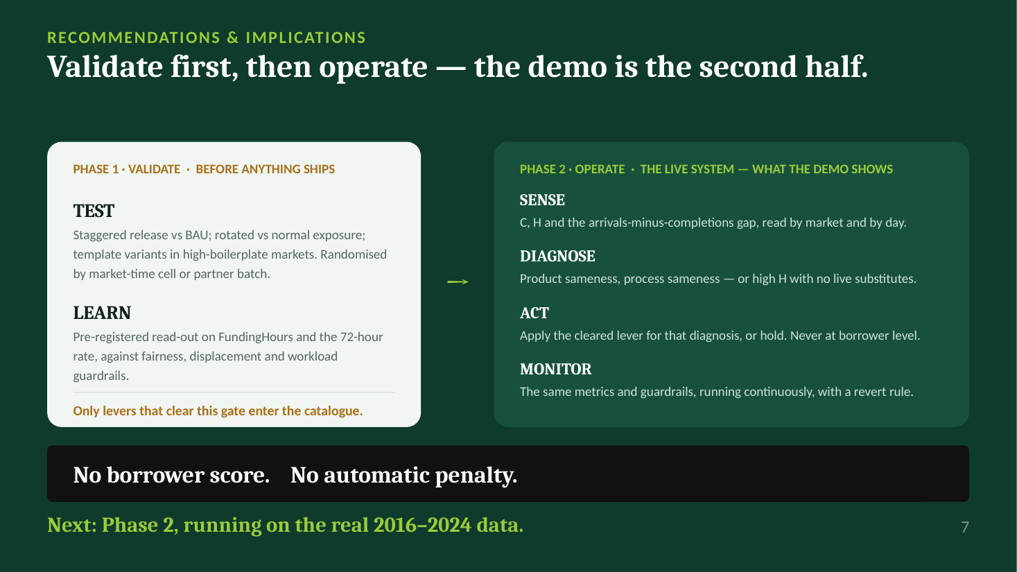 The recommendation — validate first, then operate
The full deck → — 9 slides plus 11 appendix slides carrying the model equation, the specification checks, the boilerplate detection rule, the year-by-year regime shift, and the sources.
Go deeperEverything behind this page
- The full report — scope, measurement design, three findings, heterogeneity, holdout, recommendations, limitations. Chinese original
- Simulation validation — all 14 components scored, plus a section on what the simulation cannot answer
- 42 result tables and 8 figures, each figure paired with its source CSV
- The 18-step pipeline — from a static opcode audit of the source pickle through to the packaged deliverable
- 18 source modules and the runbook
- The review log — independent review rounds, including the ones that failed